
Why are financial markets so unpredictable?
Financial problems are difficult to predict. The stock market is well organized and contributes to job creation as a useful source of business financing, but it is also fraught with risk. In the foreign exchange market, traders convert dollars into euros, yen, rubles, or pounds sterling, primarily to make a small percentage of profit on a very large transaction. Professional traders and traders use their experience to keep the risk as low and the profit as high as possible.
But the stock market is more complex than horse racing, and traders now rely on complex algorithms that are mathematical models running on computers. Many trades have been automated: algorithms make split-second decisions and trade without any human intervention.
All of these developments are motivated by the desire to make financial problems more predictable, reduce uncertainty, and thus reduce risk. The financial crisis happened precisely because too many bankers thought they had done so. As it turns out, they might as well have looked into a crystal ball.
This is not a new problem.Between 1397 and 1494, in Renaissance Italy, the powerful Medici family ran a bank that was the largest and most respected in all of Europe. At one time it made the Medici family the richest in Europe. in 1397, Giovanni di Bicci de’Medici spun off his own portion of his nephew’s bank and moved it to Florence. The bank continued to expand, with branches in Rome, Venice, and Naples, before spreading its tentacles to Geneva, Bruges, London, Pisa, Avignon, Milan, and Lyon. All seemed to be going well under the rule of Cosimo de’Medici until his death in 1464, when his son Piero took over.
Behind the scenes, however, the Medici family was a profligate spendthrift: from 1434 to 1471, they spent around 17,000 gold florins a year. This is the equivalent of 20 to 30 million dollars today.
Hubris begets retribution, and the inevitable collapse began with the Lyon branch, which had a dishonest manager. The London branch then made a large loan to the ruler of the time, a risky decision given that the king and queen were somewhat unpredictable and had a reputation for not repaying their debts, and in 1478 it collapsed with a total loss of 51,533 gold florins. The Bruges branch made the same mistake. According to Niccolo Machiavelli, Piero tried to shore up the finances by taking on debt, which in turn put several local businesses out of business and annoyed many influential people.
Branch after branch failed, and when the Medici family fell out of favor and lost political influence in 1494, the end was in sight. However, even though the Medici were still the largest bank in Europe at that time, a mob razed the central bank in Florence and the Lyon branch was subject to a hostile takeover. The manager of Lyon had approved too many bad loans and borrowed heavily from other banks to cover up the disaster.
This all sounds very familiar: during the dot-com bubble of the 1990s, when then-Federal Reserve Chairman Alan Greenspan gave a speech in 1996 decrying the market as “irrationally exuberant,” investors sold off their vastly profitable brick-and-mortar properties and gambled them against what groups of kids could whip up in their attics with their computers and modems. as “irrational exuberance”. But no one cared until the dot-com crash of 2000. By 2002, a total of $5 trillion had been lost in market capitalization.
It’s happened many times before. 17th-century Holland was prosperous and confident, and it reaped huge profits from trade with the Far East. Tulips, a rare flower from Turkey, became a status symbol, and their prices soared, leading to a “tulip mania” that spawned a specialized tulip exchange. Speculators buy stock and hold it in their hands, creating artificial scarcity to drive up prices. A futures market for contracts to buy and sell tulips at a future date was created. By 1623, a rare tulip cost more than an Amsterdam merchant’s house. When the bubble burst, the Dutch economy was set back 40 years.
In 1711, British entrepreneurs formed a company to “manage and co-ordinate the merchants of Great Britain in the trade of the South Pacific and other parts of America, and also to encourage the fisheries”. The British king granted it a monopoly on South American trade. Speculators drove up the price tenfold, and a series of bizarre spin-off companies were formed. One very famous prospectus said, “In a business with great advantages, but no one knows exactly what.”
Again, this is nonsense. When sanity was restored, the market collapsed: ordinary investors lost their life savings, while major shareholders and directors had long since fled the market. In the end, it took Robert Walpole, the first British Treasury Minister, who sold off all his shares at the peak and split the debt between the government and the East India Company, to restore order. Directors were forced to compensate investors, but many more of the worst offenders remain at large.
When the financial bubble burst, Newton, then director of the Mint, hoping to use it to understand high finance, commented, “I can calculate the motion of the stars, but not the madness of mankind.” It took quite some time before mathematically minded academics began to study market mechanisms, and in the meantime, they even began to focus on how to make rational decisions, or at least make the best estimates of which behaviors are rational.
The Underrated Brownian Motion Model
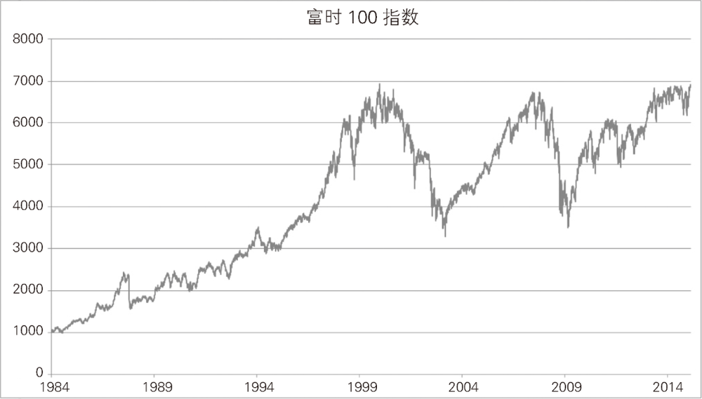
Anyone who reads the financial pages of a newspaper or follows the stock market on the internet will quickly realize that the volume and price of stocks can change in an irregular and unpredictable way. Figure 1 shows how the FTSE 100 index (the composite price of the top 100 companies on the UK stock market) has changed between 1984 and 2014. It looks more like a random walk than a smooth curve.
Baselier discovered this similarity and used a physical process called Brownian motion to model changes in share prices. in 1827, the Scottish botanist Robert Brown, while looking through a microscope at particles in the cavities of pollen grains suspended in water, noticed that the particles were randomly shaking, but was unable to explain why. in 1905, Albert Einstein proposed that particles collide with water molecules. water molecules were colliding. His mathematical analysis of this physical phenomenon led many scientists to believe that matter was made up of atoms (a surprisingly controversial concept in 1900.) In 1908, Jean Perrin confirmed Einstein’s explanation.
Using the Brownian motion model, Baselier answered a statistical question about the stock market: how do expected prices (statistical averages) vary over time? Specifically, what does the probability density of prices look like? And how does it evolve?
Baselier gave an estimate of the most likely future price, and the range of possible fluctuations relative to that price. He provided a probability density equation now known as the Kolmogorov-Chapman equation and solved it to obtain a normal distribution whose variance (spread) increases linearly over time.
We now know that this is the probability density of the diffusion equation, and this equation is also called the heat transfer equation because that’s where it first appeared. If you heat a metal pan on the stove, the handle gets hot, even though it is not in direct contact with the heat source, because the heat diffuses through the metal. 1807, Fourier gave a “heat conduction equation” that governs this process. The same equation applies to other types of diffusion, such as the diffusion of a drop of ink in water. Baselier proved that in the Brownian motion model, the price of an option spreads like heat.
He also developed a second method using random walks. If the random walk is taken at smaller and smaller paces and at faster and faster speeds, it can be approximated as Brownian motion. He noted that this concept would give the same result. He then calculated how the price of a “stock option” should change over time (A stock option is a contract to buy or sell a commodity at a fixed price at a future date. These contracts can be bought and sold, and the appropriateness of the purchase or sale depends on the actual price movement of the commodity). By understanding how the current price spreads, we can get the best estimate of the actual future price.
The paper had a lukewarm reception, probably because it had a less common field of application, but it passed and was published in a high quality scientific journal. Baselier’s career was then ruined by a tragic misunderstanding. He continued to study diffusion and related probabilistic topics and became a professor at the Sorbonne in France, however, when World War I broke out, he joined the army. After the war, and after some temporary academic work, he applied for a permanent position in Dijon.
Maurice Gevrey, who was responsible for evaluating the application, thought he had found a major error in one of Baselier’s essays, which was echoed by expert Paul Levy. Bachelier’s career was ruined. But they both misunderstood his notation; it was not wrong. Baselier wrote a letter of righteous indignation about it, but to no avail. Eventually Levi realized that Baselier had not been wrong all along, and after apologizing, they made up. Even then, however, Levi never became interested in the application of the paper to the stock market. He commented on the paper in his notebook, “So much about finance!”
Baselier’s analysis of how the value of stock options changes over time using stochastic fluctuations was eventually embraced by mathematical economists and market researchers. The goal was to understand the behavior of the market in which options (not just the underlying commodity) are traded. A fundamental problem was to find rational ways to price options, that is, **everyone could use the same rules to figure out prices for the things they cared about separately. ** This makes it possible to assess the risk involved in a particular trade, and thus incentivizes market activity.
The Overrated Black-Scholes Pricing Model
In 1973, Fischer Black and Myron Scholes published “Options and Corporate Debt Pricing” in the Journal of Political Economy. Over the previous decade, they had developed a mathematical formula to determine a reasonable price for a given option. Experiments with trading using this formula were not very successful, so they decided to make their reasoning public. Robert Merton provided a mathematical explanation of their formula, which came to be known as the Black-Scholes option pricing model. It distinguishes fluctuations in the price of an option from the risk of the underlying commodity, leading to a trading strategy known as delta hedging: In a sense, repeatedly buying and selling the underlying commodity to eliminate the risk associated with the option.
The Black-Scholes model is a partial differential equation, known as the Black-Scholes equation, which is closely related to the diffusion equation that Baselier distilled from Brownian motion. Numerical methods can be used to find the optimal price of an option in any situation. The fact that a single “reasonable” price could be calculated (even though it was based on a specific model that might not be applicable in reality) was enough to convince financial institutions to use it, and a huge options market was born.
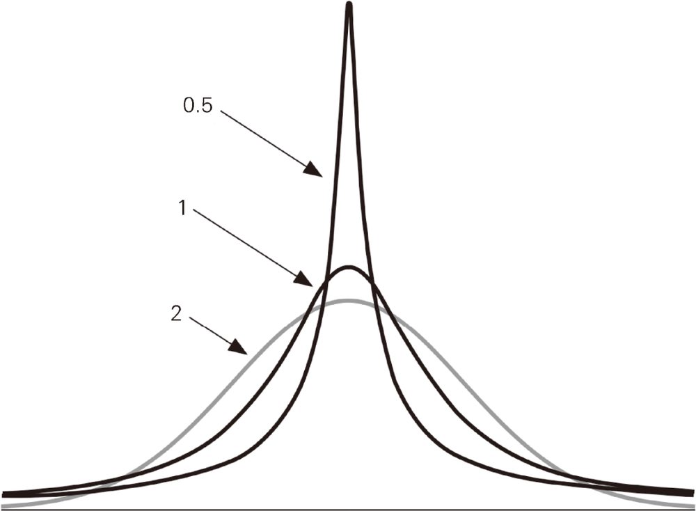
The mathematical assumptions used in the Black-Scholes equation are not entirely consistent with reality. One important reason is that the probability distribution of the implied diffusion process is normal, so extreme events are unlikely to occur. In fact, such events are much more common, a phenomenon known as thick tails. There is a class of probability distributions known as stable distributions that are made up of four parameters, three of which are shown in Figure 2, with each of their key parameters corresponding to a specific value. When this parameter is 2, we get the normal distribution (gray curve), which has no thick tails. The other two distributions (black curve) have thick tails: on both sides of the graph, the black curve is above the gray curve.
The black curve is above the gray curve on both sides of the graph.
Using a normal distribution to model financial data that actually has thick tails greatly underestimates the risk of extreme events. With or without thick tails, these events are rare compared to normal, but the thick tails make them common enough to pose a serious problem. Of course, extreme events can cost you a ton of money. Unexpected shocks, such as sudden political upheaval or the collapse of a large company, can make extreme events more likely than the thick-tailed distribution would predict. The Internet bubble and the 2008 financial crisis were both associated with such unexpected risks.
Despite these problems, the Black-Scholes equation is widely used for its utility: it is easy to calculate and most of the time gives a good approximation of what happens in the real market. Billionaire and investor Warren Buffett has warned that “the Black-Scholes equation is as close to sacred as you can get in finance. …… However, if the equation is applied over longer time periods, it can lead to absurd results. To be fair, Black and Scholes must have understood this. But their devoted followers may have overlooked the cautionary note that accompanied the formula when they both first publicized it.”